Coordinate Compression
[out:json][timeout:3600];
area["ISO3166-1"="DE"][admin_level=2];
way["highway"]["surface"~"^(gravel|fine_gravel|compacted|pebblestone)$"](area);
out skel geom;
Return all gravel roads 1 in Germany and their geometry. This innocent-looking Overpass query forced Node.js to its knees. "Cannot create a string longer than 0x1fffffe8 characters", it whispered with its dying breath. Limited to an internal string length of 512 MB, it was not prepared to deal with the data flooding in.
I had to switch the response type to stream and use the stream-json library to parse it. The result measured 614 MB, despite only containing basic structural skel and geometric geom information. I stripped it down even further to just the polylines. 240 MB and 1,032,029 polylines with an average length of 10.15 coordinates, to be exact.
[
  // [longitude, latitude]
  [9.5720777, 51.8684697],
  [9.5713593, 51.8682805],
  [9.5709083, 51.8681333],
  [9.5705485, 51.8679984],
  [9.5703925, 51.8679399]
]
614,312 KB -> 239,784 KB
Simplify
The first two rounds of compression are lossy. The polylines are more detailed than necessary, so we drop as many coordinates as possible. There are a couple algorithms to choose from. One of them is Douglas–Peucker. It recursively divides a polyline into segments by including the most distant point from the current segment until all points are either included or within a given tolerance.
Here are some examples of different tolerances applied to the same polyline:
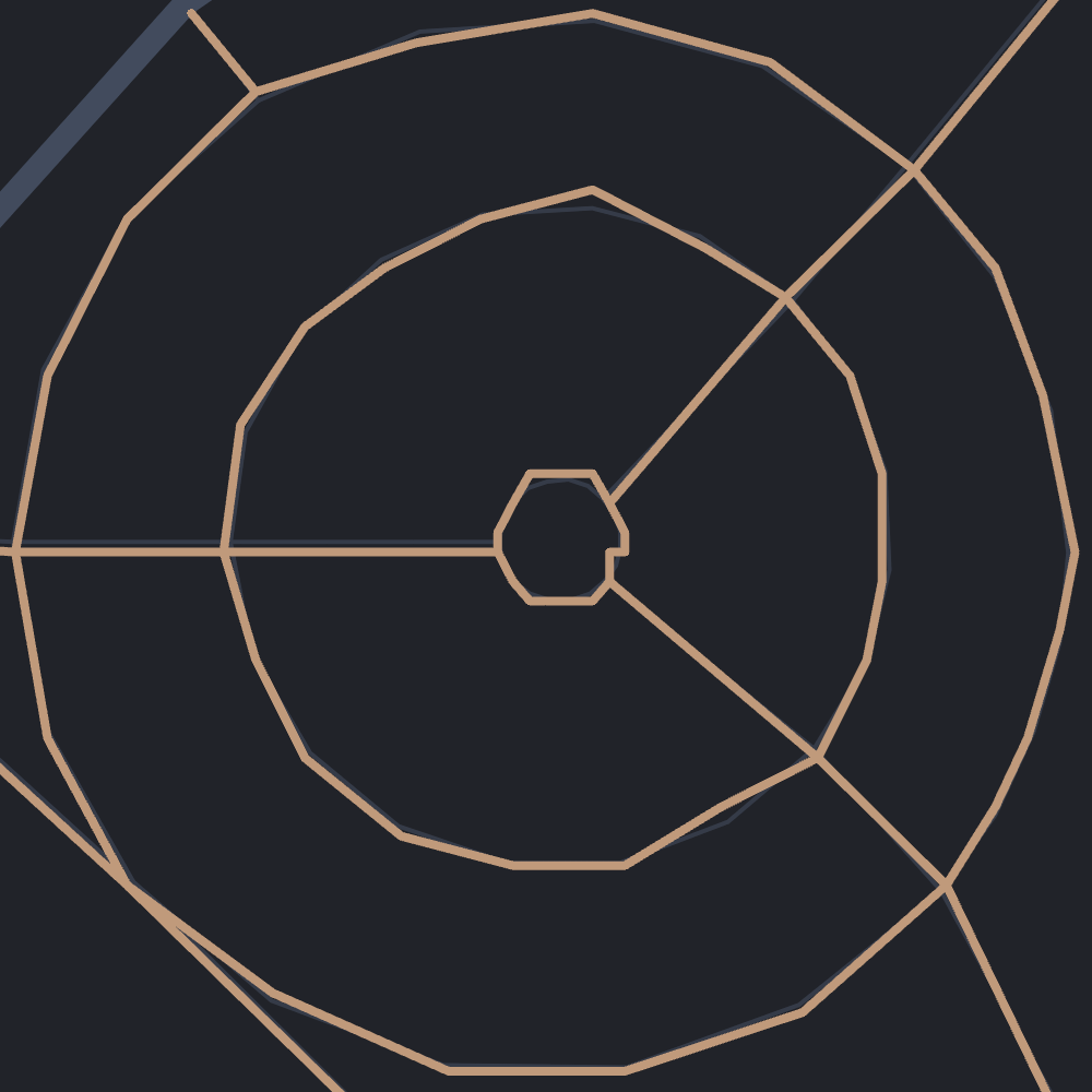
Full detail 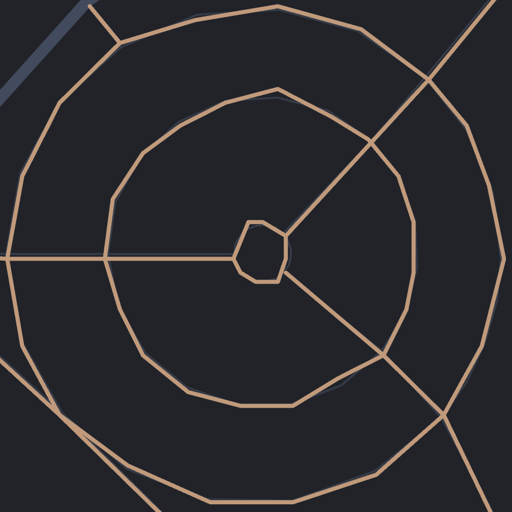
Tolerance of 0.5 meters
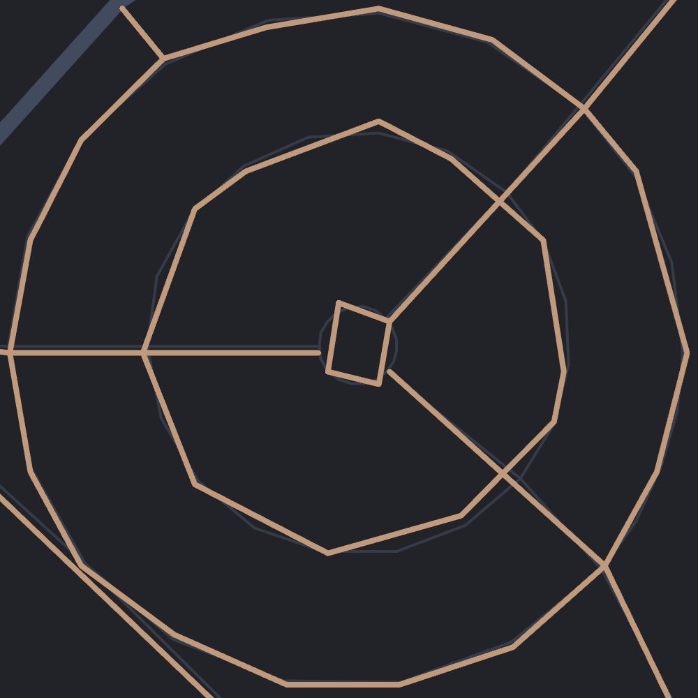
Tolerance of 1 meter 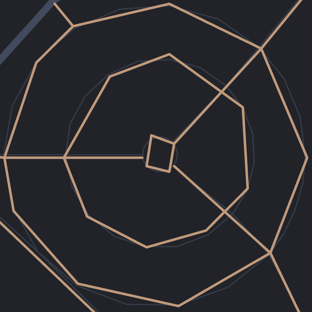
Tolerance of 2 meters
I chose the 0.5 meters tolerance because it still looks smooth and close to the original. Using it decreased the average polyline length by around 20% to 8.3 coordinates.
[
  [9.5720777, 51.8684697],
  [9.5713593, 51.8682805],
  [9.5709083, 51.8681333],
  // Removed [9.5705485, 51.8679984]
  [9.5703925, 51.8679399]
]
239,784 KB -> 196,512 KB
Precision
The second lossy compression step concerns the precision of coordinates. More decimal places mean higher precision but also more data. The following relation between decimal places and precision applies to latitudes:
| DD.dddddd° | Decimal places | Meters |
|---|---|---|
| 1° | 0 | 111,120 |
| 0.1° | 1 | 11,112 |
| 0.01° | 2 | 1,111.2 |
| 0.001° | 3 | 111.12 |
| 0.0001° | 4 | 11.112 |
| 0.00001° | 5 | 1.1112 |
| 0.000001° | 6 | 0.11112 |
| 0.0000001° | 7 | 0.011112 |
Longitudes have the same precision at the equator and get more accurate closer to the poles as the distance between meridians decreases. So the values in the table above are the worst case in terms of precision. The obvious choice here is five decimal places, because it's neither too coarse nor too fine.
[
  [957208, 5186847], // [round(9.5720777 * 1e5), round(51.8684697 * 1e5)]
  [957136, 5186828], // [round(9.5713593 * 1e5), round(51.8682805 * 1e5)]
  [957091, 5186813], // [round(9.5709083 * 1e5), round(51.8681333 * 1e5)]
  [957039, 5186794]  // [round(9.5703925 * 1e5), round(51.8679399 * 1e5)]
]
196,512 KB -> 148,188 KB
Offset
Now come the lossless compression steps. Coordinates in polylines are usually within close proximity, so it makes sense to store the offset to their predecessor instead of the full coordinate.
const previous = [0, 0];

function offset(coordinates) {
  return coordinates.map((coordinate, index) => {
    const offset = coordinate - previous[index];
    previous[index] = coordinate;
    return offset;
  });
}
They are calculated across polyline boundaries. For the offset of a polyline's first coordinates, the previous polyline's last coordinates are used. As a result, the order of polylines has a minor influence on the compression efficiency. Here are four options to sort them:
- Random
- Sort output by quad tile
out qt; - Sort polylines by nearest neighbor
- Sort polylines optimally
Option four is impossible for the data size, because it resembles the infamous traveling salesman problem and thus is NP-hard. The second best option, sorting by nearest neighbors, yields a minor compression improvement compared to the others and also takes some load off the Overpass server because it doesn't need to sort itself.
[
  [240, 356], // [957208 - 956968, 5186847 - 5186491]
  [-72, -19], // [957136 - 957208, 5186828 - 5186847]
  [-45, -15], // [957091 - 957136, 5186813 - 5186828]
  [-52, -19]  // [957039 - 957091, 5186794 - 5186813]
]
148,188 KB -> 72,932 KB
Zigzag
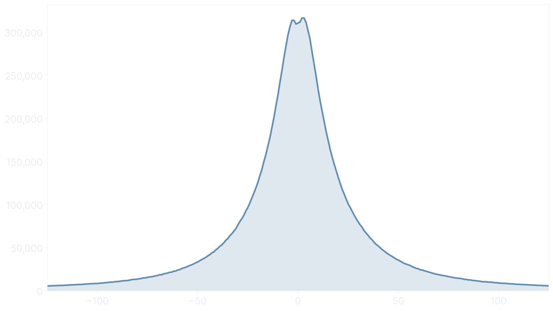
This step acts as preparation for the binary encoding. We need to convert signed integers to unsigned ones while preserving a one-to-one mapping. To achieve that, we use the zigzag algorithm. If the offset is positive, we zig offset * 2 , otherwise we zag -offset * 2 - 1.
function zigzag(offset) {
  return offset >= 0 ? offset * 2 : -offset * 2 - 1;
}
The encoding also works best with small numbers. Fortunately, small offsets are the most frequent in polylines by nature, so there is no reason to use a more complicated alternative like Huffman coding.
[
  [480, 712], // [240 * 2, 356 * 2]
  [143,  37], // [72 * 2 - 1, 19 * 2 - 1]
  [ 89,  29], // [45 * 2 - 1, 15 * 2 - 1]
  [103,  37]  // [52 * 2 - 1, 19 * 2 - 1]
]
72,932 KB -> 69,300 KB
Encode
In the last step, we convert the zigzagged offsets into binary data. For that, we use variables integers, a base-128 integer encoding that can, as the name suggests, span a variable number of bytes depending on its size. The lower bits of a byte contain the data, while the upper bit defines whether or not the integer continues in the next byte. Compared to other encodings, small numbers take up very little space, which makes it ideal for our use case.
function writeVarint(out, value) {
  while (value > 0x7f) {
    out.push((value & 0x7f) | 0x80);
    value >>>= 7;
  }
  out.push(value);
}
We also need to include the polyline's length in the encoded data. Otherwise we wouldn't know when to stop once we get to decoding.
0x04,       // Length: 4
0xe0, 0x03, // 1 lng: (480 & 0x7f) | 0x80, (480 >>> 7) & 0x7f
0xc8, 0x05, // 1 lat: (712 & 0x7f) | 0x80, (712 >>> 7) & 0x7f
0x8f, 0x01, // 2 lng: (143 & 0x7f) | 0x80, (143 >>> 7) & 0x7f
0x25,       // 2 lat: 37
0x59,       // 3 lng: 89
0x1d,       // 3 lat: 29
0x67,       // 4 lng: 103
0x25        // 4 lat: 37
69,300 KB -> 20,390 KB
Conclusion
We have reached the end. I can't think of any other way to improve the compression. Now all that's left to do is zip up the data, which leaves us at 18 MB, a 97% reduction relative to the raw data. If we compare it to Google's polyline codec, our custom one is around 20% smaller.
Here is a recap of each step with its corresponding size:
| Step | Description | Size [KB] |
|---|---|---|
| Raw | Raw data returned by the Overpass API | 614,312 |
| Geometry | Remove all but geometric data | 239,784 |
| Simplify | Simplify polylines with a tolerance of 0.5 meters | 196,512 |
| Precision | Round coordinates to 5 decimal places | 148,188 |
| Offset | Store offset to previous coordinates | 72,932 |
| Zigzag | Convert signed to unsigned integers | 69,300 |
| Encode | Encode using variable integers | 20,390 |
| Compress | Compress using deflate | 17,501 |
But with great datasets come great performance problems. To be continued.
Gravel isn't well defined by the community, so I used my would-I-ride-that metic while looking at OpenStreetMap's unpaved surfaces.↩︎